Batch Gradient Descent in Linear Regression with Multiple Variable

一、参考资料

1. 深入梯度下降(Gradient Descent)算法
2. 梯度下降（Gradient Descent）小结(by 刘建平Pinard)

二、代码实现

import pandas as pd
import numpy as np


#读入训练数据与测试数据
df_train = pd.read_csv('train_data.txt', sep='\t', header = None)
df_test = pd.read_csv('test_data.txt',sep = '\t',header = None)

#将测试数据与训练数据数组化
train_array = df_train.values
test_array = df_test.values

#记录训练数据每一列的的最大最小值
train_array_max = []
train_array_min = []

#归一化训练数据和测试数据
for i in range(train_array.shape[1]-1):
    train_array_max.append(np.max(train_array[:,i]))
    train_array_min.append(np.min(train_array[:,i]))
    #print(train_array_max[i],train_array_min[i])
    train_array[:,i] = (train_array[:,i]-train_array_min[i])/(train_array_max[i]-train_array_min[i])
    test_array[:,i] = (test_array[:,i]-train_array_min[i])/(train_array_max[i]-train_array_min[i])

#拼接训练数据
#n组训练数据，m个参数
n = train_array.shape[0]
m = train_array.shape[1]

x = np.hstack((np.ones([n,1]),train_array[:,:m-1].reshape(n,m-1)))
y = train_array[:,m-1].reshape(n, 1)

#print(y.T.shape)
#print(x)
#print(y)
#print(n)

#存放系数矩阵
h0 = np.zeros([1,m])
h = np.zeros([1,m])
J = np.sum((x.dot(h0.T)-y)**2)/(2*n)

#print(h0)
#print(h0.T)
#print(J)
# print(x.shape[0],x.shape[1])
# print(y.shape[0],y.shape[1])
# print((x.dot(h0.T)-y).shape[0],(x.dot(h0.T)-y).shape[1])
# print((x[:,0].reshape(n,1)).shape[0],(x[:,0].reshape(n,1)).shape[1])
# print(((x.dot(h0.T)-y)*x[:,j].reshape(n,1)).shape[0],((x.dot(h0.T)-y)*x[:,j].reshape(n,1)).shape[1])

J0 = 0
a = 0.01
loss = []
import copy
#BGD
while np.abs(J-J0) > 1e-3:
    loss.append(J)
    J0 = J
    for j in range(m):
        #print(np.sum((x.dot(h0.T)-y)*x[:,j].reshape(n,1))/n)
        h[0][j] = h0[0][j] - a*np.sum((x.dot(h0.T)-y)*x[:,j].reshape(n,1))/n
    h0 = copy.deepcopy(h)
    J = np.sum((x.dot(h0.T)-y)**2)/(2*n)

#梯度下降过程中损失的变化趋势
import matplotlib.pyplot as plt
plt.plot(np.arange(len(loss)), loss)
plt.show()

#训练数据预测值与真实值进行比较
pre_y = x.dot(h.T)
plt.plot(np.arange(len(y)),y,pre_y)
plt.show()

#预测测试数据
tn = test_array.shape[0]
test_x = np.hstack((np.ones([tn,1]),test_array[:,:m-1].reshape(tn,m-1)))
test_y = test_array[:,m-1].reshape(tn,1)
pre_test_y = test_x.dot(h.T)

#预测值与真实值进行比较
plt.plot(np.arange(len(test_y)), test_y,pre_test_y)
plt.show()

三、实验结果

四、其他实例

1. 题目

2. 数据

train_data: 传送门

3. 代码

import pandas as pd
import numpy as np

data = pd.read_csv('data1a.txt', header=None)
data = data.values


# n 表示特征数，m 表示样本数
# print(data_x.shape)
n = data.shape[1] - 1
m = data.shape[0]

# data_x 为输入特征, data_y 为目标结果
data_x = data[:, 0 : -1].reshape(m, n)
data_x = np.concatenate((np.ones([m, 1]), data_x), axis = 1)
data_y = data[:, -1].reshape(m, 1)


# print(data)
# print(data_x)
# print(data_y)
theta = np.zeros([n+1, 1])
# print(theta)

# 计算假设函数
h = data_x.dot(theta)

#计算损失函数
J = np.sum((h-data_y)*(h-data_y))/(2*m)

# print(J)

alpha = 0.01
J0 = 0
loss = []

print("Initial Loss: ", J)

while abs(J-J0) > 0.00001:
    loss.append(J)
    J0 = J
    for i in range(0, n+1):
        delta = alpha*np.sum((h-data_y)*data_x[:, i].reshape(m,1))/m
        theta[i][0] = theta[i][0] - delta
    h = data_x.dot(theta)
    J = np.sum((h-data_y)*(h-data_y))/(2*m)
#     print(J)

print("Fianl Loss: ", J)
print("Fianl theta: ", theta[0][0], theta[1][0])

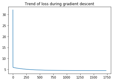
#梯度下降过程中损失的变化趋势
%matplotlib inline
import matplotlib.pyplot as plt
plt.plot(np.arange(len(loss)), loss)
plt.title("Trend of loss during gradient descent")
plt.show()


test_x = np.ones([2,2])
test_x[0][1] = 3.5
test_x[1][1] = 7

test_y = test_x.dot(theta)

print("A, B 的利润分别为: ", test_y[0][0], test_y[1][0])

Initial Loss:  32.072733877455676
Fianl Loss:  4.479729514503939
Fianl theta:  -3.7217231514189435 1.175547657550631

A, B 的利润分别为:  0.39269365000826495 4.507110451435473